Help for CPO Programs

Test2d01, 1st 'benchmark test' data file for CPO2D

Idealised hemispherical deflection analyzer (HDA)

Here an idealised hemispherical deflection analyser is created out of two complete concentric spheres. Examples are shown of the potentials and fields in the space between the spheres. A ray is then started with the median energy along the median path. The final coordinate at the exit plane, which should be 1.0, can be seen to be 0.99996.

The number of segments used in the present example is small enough for the example to be run with the ‘demo’ version of CPO2D. Higher accuracy could of course be obtained with more segments, using the standard or full versions of CPO2D.

Detailed description:

The radii of the hemispheres are 0.75 and 1.25, and the numbers of subdivisions for the 2 hemispheres (15 and 25) have been chosen to be approximately proportional to their radii, as recommended.

The requested inaccuracy for the potentials and fields is 0.001.

The following data were obtained when the memory and speed of PC's was much more limited than at present, so the available number of segments was small and the requested inaccuracies were fairly high to give a quick demonstration.

The potentials of the hemispheres are such that the potential at the mid-radius (r = 1) should be 1 and the field should be 2. More generally, the potential is 2/r-1 and the field is 2/r**2 (see detailed equations on HDA). The calculated values at various points between the spheres appear on the screen and in the output data file (tmp1a.dat), and are consistent with the requested inaccuracy, to within a factor of about 2 (the typical inaccuracy being 0.0005).

The following table gives a small sample of results, to illustrate how the average inaccuracy (err) in the potential at the mid-radius depends on (1) the total number (N) of segments, and (2) the requested inaccuracy (acc_pot) for the evaluation of the potentials and fields. The fourth column shows the product of the error and the square of N (and the square has been chosen empirically, because it leads to approximately constant values of the product under some conditions). The fifth column shows the factor that seems to be limiting the error.

N        acc_pot        err                err*N^2        limiting factor

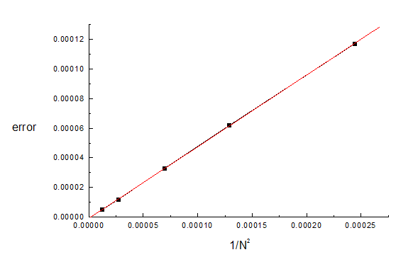
288        0 .00001        0.000005        0 .41                N

192        0 .00001        0.000012        0 .44                N

120        0 .00001        0.000033        0 .48                N

88        0 .00001        0.000062        0.48                N

64        0.00001        0.000117        0 .48                N

192        0 .0001        0.000021        0 .77                acc_pot

120        0.0001                0.000044        0 .63                acc_pot

88        0.0001                0.000073        0.57                N,acc_pot

64        0.0001                0.00013        0.53                N,acc_pot

40        0.0001                0.00030        0.48                N

24        0.0001                0.00082        0.47                N

It can be seen that when N is limiting factor the errors in the potentials are approximately proportional to 1/N^2. For example here is the plot of the error versus 1/N**2 for the first 5 lines of the table:

The errors in the fields have the same dependence and approximately the same magnitude. Note that when the limiting factor is acc_pot, the inaccuracy is usually less than the requested value of acc_pot. The empirical dependence on N allows the results to be extrapolated to N = infinity, as described in Chapter 3 of the User's Guide.

The ray starts at r = 0, z = -1. The requested inaccuracy for the ray tracing (acc_traj, say) has been set at .001, the initial step length is 0.1 (to ensure a smooth ray plot at the start of the ray, see the relevant note), and the maximum step length (step_max, say) has been set at 0.3 (see below). The value of z at the exit plane (r = 0, which has been specified as a 'test plane') should be +1.0, and in this example is 0.99996 (see the output data file 'tmp1a.dat'), giving an error of 0.0011 (which is consistent with the requested ray inaccuracy of 0.001).

This error is easily improved (to 0.00004 in the present example) by using the 'total energy' option instead of the 'kinetic energy' option (see the relevant note). The difference is due to the fact that the median ray is given the kinetic energy = 1eV, and it should start with a potential energy = -1eV, and therefore a total energy of 0eV, but the calculated initial potential will not be exactly 1.0. With the 't' option the user inputs the value 1.0 for the initial potential, and then the program makes the necessary adjustment to the potential everywhere in the system, so that the total energy (a constant of motion) will be exactly 0eV. But note that for the inexperienced user the 't' option can easily be misused, giving misleading results, and so it has not been employed in the present data file.

Four other rays are also entered, with initial angles of +/-0.1 radians and +/-0.2 radians in the dispersion plane. At the exit plane the first 2 should have z=0.9803 and the second 2 z=0.9241 (see 'equations' in Help); the computed values differ from these by typically 0.0010, which is again consistent with the requested inaccuracy.

The option to choose the colours of the rays is demonstrated here. The option is activated by putting 'col' in spaces 21 to 23 of the line that specifies the type of rays. This is then followed by an extra line that gives the repetition number (in this case 5) and the numbers of the colours that are to be repeated (in this case the colour numbers are 1, 2, 2, 4 and 4, corresponding to blue, green, green, red and red respectively). If further rays were to be used they would repeat this sequence of colours.

This ray error depends on the values of acc_traj and step_max.

The value of acc_traj obviously represents the minimum error, but the actual error might be larger if step_max is not well chosen.

If step_max is too large the interpolation to find the values of the coordinates and velocities at the exit plane will be inaccurate (unless by chance the end point of a ray step happens to be near the exit plane).

In the present example (for which the scale length is 1) it is found empirically that the 'exit plane interpolation error' for z can be as high as of the order of 0.03*step_max**7 (that is, it is of the order of 0.0008 for a step length of 0.6). For other simulations the dependence on the step length might be quite different, eg this type of interpolation error might be negligible for a simulation in which the rays are nearly straight at the exit.

Using the 'mesh' method of ray tracing, with a mesh spacing of 0.03 (and the other parameters as in the middle line of the above table), gives essentially the same error but takes about twice as long. However, further rays that are close to this first one are much quicker. The mesh method is the more efficient, in this example, if about 3 or more closely spaced rays are required.

To obtain 100 full rotations of the electron, take the following steps:

(1) Use the mesh method, with mesh spacing 0.03 (note 18)

(2) Change the minimum r of the ray to -1.5 (note 21)

(3) Set the maximum time to 1.1E-3 (note 23), to stop the ray tracing at about 100 rotations

(4) Put the letter 'm' in the 6th space in the line that gives the number of test planes, to signify that multiple crossings are required

(5) Add 200 in the next 2 lines (after the values of a, b and d), to give the number of crossings of each plane before the crossing information is retained (and note that each plane is crossed twice in each full rotation)

(6) Use a single ray, the median ray.

You will then see in the output file (tmp1a.dat) that after 100 full rotations the final value of z at r = 0 is 0.975, a surprisingly good result.

Dec 2012: Put in latest format, after introduction of magnetic option (and due to the many changes made since this data file was first constructed, some of the above footnotes might be slightly different now).

March 2013: To test relativistic corrections, put electron kinetic energy = 511 keV (the rest mass energy, call it T0). The electric field at the median radius r should then be E, where e*E = m*v**2/r (where m is the relativistic mass).

Now m*v**2 = (T**2 - T0**2)/T, where T = T0 + kinetic energy, which in the present example gives m*v**2 = 1.5*T0. We therefore need E = (1.5*511 kV)/r. We also need a median potential of 511 kV. This field and median potential are produced by setting the potentials of the inner and outer spheres at 1.5*511 kV and 0.7*511 kV respectively (766.49 kV and 357.70 kV).

If the motion were non-relativistic, these potentials would be simply scaled up from the 1 eV case, namely 1.6667*511 kV and 0.6*511 kV (851.66 kV and 306.60 kV), giving E = (2*511 kV)/r.

Note that the factor 2 in this equation is larger than the factor 1.5 in the analogous relativistic equation because as the energy becomes more relativistic v**2 decreases faster than m increases. Alternatively, use the voltages and energies given in the footnotes of test2d22.dat.