Help for CPO Programs

Test3d01, 1st 'benchmark test' data file for CPO3D

Idealised hemispherical deflection analyzer (HDA)

Here an idealised hemispherical deflection analyser is created out of two complete concentric spheres. Examples are shown of the potentials and fields in the space between the spheres. A ray is then started with the median energy along the median path. The final coordinate at the exit plane, which should be 1.0, can be seen to be 0.99941.

(This simulation has cylindrical symmetry and so can be solved even more quickly and accurately with CPO2D, using the data in test2d01.dat).

Detailed description:

The number of segments used in the present example is small enough for the example to be run with the 'demo' version of CPO3D. Higher accuracy could of course be obtained with more segments, using the standard or full versions of CPO3D.

The following data were obtained when the memory and speed of PC's was much more limited than at present, so the available number of segments was small and the requested inaccuracies were fairly high to give a quick demonstration.

The radii of the hemispheres are 0.75 and 1.25, and the number of subdivisions for the 2 hemispheres have been chosen to be approximately proportional to their radii, as recommended.

The requested inaccuracy for the potentials and fields (and also for the rays) is 0.1% in this example.

The potentials of the hemispheres are such that the potential at the mid-radius (r = 1) should be 1.0 and the field should be 2.0 (see detailed equations on HDA). The first two sets of results that appear on the screen show the potentials and fields along an arc of a circle of radius 1.0 (that is, along the path of the median ray). The average error is 0.13%, and the maximum errors of the potentials and fields are 0.20% and 0.15% respectively. These errors are slightly larger than the requested inaccuracy, but the total number of segments is only 100 (as required for the 'demo' version). The influence of the number of segments is discussed below.

The next two sets of results show the potentials along arcs that lie on the surfaces of the outer and inner spheres. Here the maximum deviations from the applied potentials (0.6 and 1.6667) are 0.28% and 0.52%, and the average deviations are 0.23% This is typical of the whole of the two spherical surfaces. The largest errors in the potentials usually occur on the surfaces of the electrodes themselves. In fact in the Boundary Charge Method the maximum deviation at any point on the boundaries is a rigorous upper limit to the deviation of the potential inside the boundaries (see L. N. Yasnitski, Boundary Element Communications, vol 5, p 181-2, 1994), assuming that the errors are caused only by the charges and not by approximations used in evaluating the potentials. However one would usually expect the deviations far from the boundaries to be significantly less than those on the boundaries themselves.

The following table gives a small sample of results, to illustrate how the average inaccuracy (err) in the potential depends on (1) the total number (N) of segments, and (2) the requested inaccuracy (acc_pot) for the evaluation of the potentials and fields. The third column shows the product of err and N to the power of 1.5, an exponent that has been chosen empirically. The last column shows a provisional judgement about the main limiting factor for the error.

The results show that with two exceptions the error is approximately proportional to 1/N^1.5. Here is a plot of the error versus 1/N**1.5 for the first 6 lines of the table:

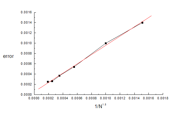
The errors in the fields have approximately the same dependence and magnitude. This dependence on N allows the results to be extrapolated to N = infinity, as described in Chapter 3 of the User's Guide.

For the value of N used in the present example, 100, we see that the expected contribution to err is approximately 0.0010.

The program is then asked to trace a ray, the median ray, through the space between the spheres. The time to do this is 10 seconds.

The value of x at the exit plane (y = 0, which has been specified as a 'test plane') should be 1.0, and in this example is 0.99941 (see the ray output file 'tmp1a.dat') -an error of 0.06%, which is consistent with the requested ray inaccuracy of 0.1% The errors can be made smaller by using the 't' option (for 'total' energy, but this option has not been included in the lines of the given data file because of ease of misuse). In this option the user would input the value 1.0 for the initial potential, and then the program would make the necessary adjustment to the potential everywhere in the system, so that the total energy (a constant of motion) would be exactly 0eV.

Using the 'mesh' method of ray tracing, with a mesh spacing of 0.05, gives approximately the same inaccuracy but takes approximately 50% longer. Further rays that are close to this first one would however be calculated very quickly (try this by repeating the data line a few times above for the first ray).