Section 3.3 of the User's Guide for CPO2D and CPO3D
(or proceed to section 3.4)
Extrapolating to infinity.
Perfect answers would be obtained for an infinitely large number of segments and for zero values of the 'charge inaccuracy', the 'ray inaccuracy', the ray step lengths or times, etc. We describe in this section a technique that gives an approximate extrapolation to these limits, and at the same time gives more reliable estimates of the errors in the final results. The technique does not require much extra computing time -the total time is usually approximately doubled or tripled.
More detailed information on extrapolating the number of segments to infinity, with the emphasis on extrapolations of 3D systems, is given in the note on extrapolation techniques for segments and in the comments on test3d15 (capacitance of a disc).
We start by considering the total number N of segments. A 'target parameter' such as a potential, a field strength, a final ray coordinate or an energy often has a power-law dependence on N. The user should establish the power law empirically, by decreasing the value of N in steps.
To illustrate this we return to the example treated in section 3.2 above. Let us pretend that the parameters given in the first row of the table below give a computing time that is as long as we can tolerate. To extrapolate N to infinity we decrease it in steps, as shown in the table:
n1 n2 N dli dlm acc_ray s
24 40 64 0.03 0.06 0.001 0.99984
18 30 48 0.03 0.06 0.001 0.99993
12 20 32 0.03 0.06 0.001 1.0001
6 10 16 0.03 0.06 0.001 1.0005
By plotting s against various powers of N we quickly find that the appropriate power for this example is approximately 1/N, as shown here:
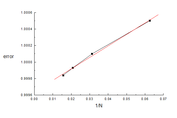
A straight line is obtained, giving an intercept of 0.99964, which therefore corresponds to an infinite value of N (and which is further away from the known value, but only small values of N have been used so far and also we have not extrapolated the other parameters yet). The change in s in going from N=64 to N=infinity is 0.00020, which can now be used as an estimated contribution to the error in s (and remember that there might be other contributions from other accuracy parameters, acc_ray, etc.).
More generally, for a power law 1/Np, and values s1 and s2 obtained at N=N1 (the highest value) and N2 respectively, the extrapolated value of s is
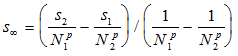
But be careful not to use this formula when N1 and N2 are too close -they should differ by a factor of at least about 2.
Similarly the dependence of s on the ray tracing inaccuracy acc_ray can be investigated (while varying the step lengths in tandem). This dependence might not be exactly linear, but it still gives a useful extrapolated value for s.
Although sinf might still not be exact after these extrapolations, it is usually a significant improvement on s1, and as a bonus the extrapolations also give an estimate of the error in s.
But note that for 3-dimensional simulations, using CPO3D, the simplest form of the technique of extrapolating N to infinity is sometimes less successful. Here the linearity of the extrapolation is often improved by increasing (or decreasing) N by a factor of 2, so that all the segments are subdivided by the same factor. A technique that is usually better is to separately extrapolate different regions -as explained in the more detailed note on extrapolation techniques.
Extrapolation can also often be used to simulate perfect accuracy for the potential and field evaluations. It is often found that the error in a potential V is approximately proportional to 1/N1.5. Capacitance calculations can also be improved, and here a power of N has been found to be 1/N. The user has to establish the appropriate power law empirically in each particular case. Some values extracted from examples mentioned in the Help menu are:
quantity p source of information
potential, field -1.5 see above, test2d01 (HDA), test3d01 (HDA)
potential, field -2 test2d15 (hole in sheet), test2d17 (mesh)
lens parameters -2 xmpl2d01, 02, 04 (lenses)
capacitance -1, -2 test3d15 (capacitance of a disc), reference list (paper in J Comp Phys)
The values of p tend to be smaller when different regions are extrapolated separately:
capacitance -0.5, -1.25 test3d15 (capacitance of a disc).
potential -0.5 see note on extrapolation techniques.
Another example is provided by the parameters of the two cylinder lens described in the ‘example’ file xmpl2d01.dat. The table shows the values obtained recently (1999, and therefore more accurate than the results presented in previous Users Guides) for the object focal length f1 of the lens (using the best available inaccuracy parameters, which are shown not to affect the results):
N = 200 300 400 600 800
f1 = 0.799716 0.799697 0.799690 0.799686 0.799684
A plot of f1 versus the inverse square of N is approximately straight, giving an intercept at f1 =0.799682 (but note that the dependence on the starting axial position has not been explored here).
If the points that correspond to the highest value of N do not lie on the straight line this indicates that the errors of those points are due to some other limitation (such as the inaccuracy of calculating the charges).
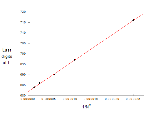
Figure 3.2 Focal length versus 1/N2 .
(proceed to next section)