Techniques for extrapolating number of segments to infinity.
As explained in chapter 3 of the Users Guide, and in several places in the Help menu, it is often possible to improve the accuracy of a result by extrapolating the number N of segments to infinity. This is achieved by using different values of N of segments (preferably differing by a factor of 4, otherwise 2) and then plotting the resulting values of the required quantity (such as potential or field) against N to the power p, where p is chosen empirically to give a straight line plot. For information on extrapolating other parameters (such as the requested inaccuracies) see chapter 3 of the Users Guide.
The appropriate values of the exponent p in the power law N**p depends on the particular quantity being extrapolated, as shown in the following table.
Values of the exponent p, from examples mentioned in the Help menu:
quantity p source of information
potential, field -1.5 chapter 3, test2d01 (HDA), test3d01 (HDA)
potential, field -2 test2d15 (hole in sheet), test2d17 (mesh)
lens parameters -2 xmpl2d01, 02, 04 (lenses)
capacitance -1, -2 test3d15 (capacitance of a disc), reference list (paper in J Comp Phys)
In practice the technique of extrapolation is usually found to be successful and reliable for 2D simulations -the plots in N**p are good straight lines. Extreme accuracy (for example better than one part per million) can sometimes be achieved for 2D problems -for example see the paper Improved Extrapolation Technique in the Boundary Element Method to find the capacitances of the unit square and cube, by F H Read, J. Computational Physics 133, 1-5, 1997 (see also the reference list). The technique in its simplest form is however sometimes less successful for 3D simulations, but then the modified technique of extrapolating separate regions is usually successful.
Here we present an example of simulation in which the simplest form of the technique is markedly less successful for 3D than 2D. It consists of a cylinder of radius 1 and length 2, plus coaxial discs of radius 1 placed at a distance of 1 from each end.
The potential of the cylinder is 0V while the two discs are at 1V. The quantity tested in the present example is the potential 0 at the centre of the cylinder.
In this example an inaccuracy of .00001 is requested for the boundary charges and potential evaluations (which was the best available before 1999). In the 3D simulation the iterative subdivision option is used with 4 stages and a 'weight' factor of 1.5. A preliminary study was used to establish that the value of 0 is most sensitive to the number of subdivisions at the ends of the cylinder. The concentrate subdivision option is therefore used for the ends of the cylinder, with a concentration factor of 5 (in detail, the concentration was applied to the 12 initial segments at an end length of 0.2 of the cylinder, while there were 12 segments on the rest of the cylinder and 12 on the disc, all the available reflection planes being used). The value of 0 is less sensitive to the number of subdivisions used for the middle part of the cylinder or for the discs.
The table shows the value obtained for
u = (0 - 0.065)*10000:
2D: N= 32 63 127 256 511
u= 4.18 2.95 2.34 2.15 2.11
3D: N= 36 63 96 126 192 256 384 508 768
u= 5.57 3.36 1.07 2.21 2.45 1.45 2.44 2.70 2.29
The figure shows the dependence of 0 on N**(-1.5).
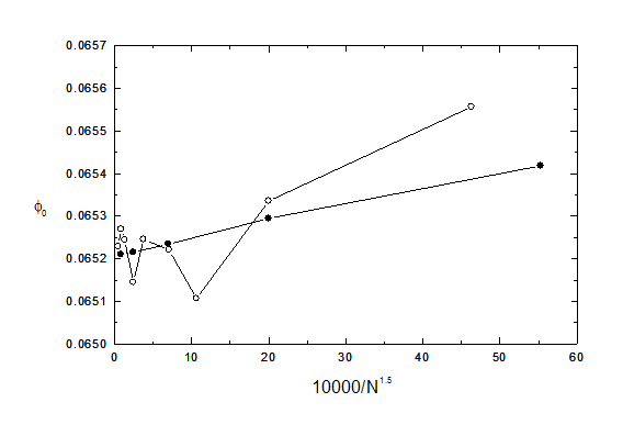
The dependence of 0 on N**(-1.5). The solid and open circles represent 2D and 3D simulations respectively.
It can be seen from the figure that the 2D results extrapolate well (as is usual), to 0.06521 0.00001. This uncertainty in the value is consistent with the requested inaccuracy of 0.00001. We can therefore state with some confidence that 0 = 0.06521 0.00002.
By contrast the 3D results do not extrapolate well (but see below). The three 3D results at the highest values of N are in the range 0.06523 to 0.06527, and so they differ from the accurate value by up to 0.00006, which is 6 times larger than the requested inaccuracy. The fluctuations are caused (see also below) by the fact that the sizes of the segments in the critical regions at the ends of the cylinder change unevenly as the total number N changes. The 3D extrapolation is worse than this (that is, the line is not straight for any value of the exponent p and the extrapolated value is less exact) if the 'concentrate subdivisions' option is not used for the ends of the cylinder. The extrapolation deteriorates further if the 'iterative subdivision' option is not used.
Another example of imperfections in the simplest form of the process of extrapolation to infinity in 3D systems is given in test3d15 (see footnotes of test3d15. The conclusion reached there is that when the extrapolation is not smooth the extrapolated result is roughly twice as accurate as the result obtained at the highest value of N.
Extrapolation of separate regions:
Another extrapolation technique is available that can be tried for 3D simulations when the technique described above is found to be unsatisfactory. This consists of identifying 2 or more regions and then carrying out separate extrapolations for the segments in them. In the present example one region consists of the ends of the cylinder and the other region is all the rest. The table shows the value obtained for u = (0 - 0.065)*10000 as the numbers of segments N1 (for the ends) and N2 (for the rest) are varied.
N1= 108 108 108 108 108 27 48 108 192 432 inf
N2= 24 96 204 384 inf 96 96 96 96 96 96
u= -5.6 2.2 4.0 5.6 9.3(3) 7.9 5.1 2.2 0.7 -0.8 -3.7(1)
These results are displayed in the figure below, where the open and solid circles represent the values for constant N1 and N2 respectively. The appropriate (empirical) exponent for these two extrapolations is now -0.5, and the extrapolations to infinity are included in the table. Using the value of 0 at N1 = 108, N2 = 96 as an 'anchor point', the change in going from N1 = 108 to N1 = infinity is -5.9 0.1 (that is, 2.2 to -3.7(1) in the table above) and the change in going from N2 = 96 to N2 = infinity is +5.7 0.3 Adding these together, the change in going to N1 = N2 = infinity is -0.2 0.3, giving u = 2.0 0.3, 0 = 0.06520 0 00003, which agrees with the value 0.06521 0.00002 given above by the 2D study.
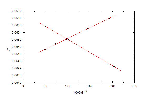
The dependence of 0 on 1/sqrt(N1) at constant N2 (solid circles) or 1/sqrt(N2) at constant N1 (open circles), where N1 is the number of segments at the ends of the cylinder and N2 is the number of segments in the rest of the system.
Note that in this example the two different regions have slopes of opposite sign for the extrapolations. The fluctuation behaviour of the open circles in the first figure can therefore perhaps be understood as resulting from a competition between opposing trends. Note also that when two or more regions are separately extrapolated fewer segments are required and the computing time is reduced. This is therefore a technique that should be used whenever possible. The table shows the empirical values that have been found for the exponent p:
capacitance -0.5, -1.25 test3d15 (capacitance of a disc).
potential -0.5 see above
The extrapolated values given above have all been deduced using a Maths package (Origin), but for routine and repeated evaluations the formula
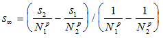
can be used, where the power law is now 1/N**p, and the values s1 and s2 are obtained at N=N1 (the highest value) and N2 respectively. But be careful not to use this formula when N1 and N2 are too close -they should differ by a factor of typically about 2.
General advice:
This example illustrates that when results of the highest ultimate accuracy are required in 3D simulations it is important to:
(1) carefully choose the initial distribution of subdivisions and either
(a) extrapolate the critical region separately from the rest, or
(b) use the 'iterative subdivision' and 'concentrate subdivisions' options.